Docking a covalently bound ligand
In this tutorial we illustrate how to re-dock the native covalent ligand of PDB id 3c9w. Both, the receptor (3cw9.pdbqt) and ligand (3c9w_ligandWithSideChain_random.pdbqt) are available in the data file associate with this tutorial.
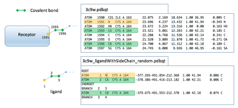
For covalent docking, the receptor and covalent ligand need to share 3 atoms as sown below. 2 atoms (green) for the covalent bond and 1 atom (yellow) is an anchor atom on the receptor side. These atoms are used to transform the ligand into place with respect to the receptor to create the covalent bond.
NOTE: for covalent docking no translational points are needed as the ligand is positioned in the docking box using the covalent bond.
In this tutorial you will learn:
- to generate a target file for covalent docking
- to run ADFR to dock the ligand
- to understand the output of an ADFR docking run
Generate the target file containing the affinity maps.
Details:
- In this example we specify the box placement and size manually to illustrate this capability. Note that this is the only -b/-boxMode option for which padding is ignored.
- The PDB serial numbers of the 2 receptor atoms forming the covalent bond are specified using the -c/–covalentBond option. The numbers are the serial codes appearing in the pdbqt file.
- The third atom defining the covalent attachment is used to compute the torsion angle of the covalent bond. It is specified using the -t/–covalentBondTorsionAtom option.
- The -x/–covalentResidues option allows to limit the traversal of the receptor to a list or residues. This is needed sometimes as covalent residues can create bonds with the receptor other than the covalent attachment and this is the case with the native ligand of 3cw9. When agfr identifies the sub-tree beyond the covalent bond to find which atoms to cut out of the receptor for calculating affinity maps, it would include a large part of the receptor because of the spurious bond the ligand makes with the receptor and cut out in excess of 1600 atoms. The -x option prevents this from happening.
- the target file is called 3c9w_cov_cmdline.trg (-o option)
The output of this commands is shown below:
Display information about a target file
Details: the target file meta data is read and displayed.
The command produces the following output:
Dock the randomized ligand using the generated target file
Details: Here we re-dock the native ligand, that has been randomized (i.e. its conformation as well as it positions and orientation in the crystal structure have been randomly modified). adfr detects the number of cores available and by default will use them all to perform 8 independent searches (–nbRuns 8) each using up to 100’000 evaluations of the scoring function (–maxEvals 100’00). By default adfr performs 50 searches, each allotted 2.5 million evaluations. Typically, more complex docking problems require more searches to be performed to increase the chances to find the best possible docked pose (i.e. global minimum of the scoring function). Here we set these parameters to lower values to perform a quick run that is sufficient to illustrate the docking principles.
This calculation generates the following files:
-
3c9w_ligandWithSideChain_random_covalent_summary.dlg # the docking log file that captures most of what is displayed on the terminal
-
3c9w_ligandWithSideChain_random_covalent_out.pdbqt # the docking pose file containing the docking solutions
-
3c9w_ligandWithSideChain_random_covalent.dro # the docking object file that contains input, output, and meta-data for this docking run
NOTES:
- The output files are named using the ligand name followed by the job name (–jobName if specified)
- ADFR’s search procedure is stochastic, meaning that docking the same ligand into the same target twice can produce different results if different random number generator seeds are used. However, the energy landscape for this receptor and ligand is the same in both runs. If both docking runs find the global minimum of this energy landscape, the solutions produced by both runs will be the same, independently of the paths taken by the search to get there. On the other hand, searches that get trapped in a local minima, yield docking poses that differ from each other. Specifying the seeds used by the random number generator (–seed) allows reproducing a docking calculation, for a given version of the code.
The output of the command is listed below:
Here we describe line by line the messages output during the docking procedure.
- Hostname and platform architecture on which the program is running
- Date and time of execution
- ligand docked
- number of detected and used cores.
- target files used
NOTES:
- Number of cores. By default ADFR will use all cores available to parallelize the search threads comprised in a run. Use the “-c” command line option to limit the number of used cores.
By default, ADFR performs 50 independent searches, i.e. 50 evolutions of a population of 100 individuals using a Genetic Algorithm (GA). In this example we intentionally reduced this number to 8 very short runs.
Lines 1-4 display a progress bar indicating the percentage of these runs that completed.
The lines below provide statistics over the termination status of these searches. ADFR implements several termination criteria in its search method. In this example all search terminated because they reached their maximum number of evaluations. The default number of evaluations is 2.5 millions and is usually never reached because of other termination criteria such as convergence of the population, meaning that there is no more diversity in the population and the chances to discover new solutions has become small, or the population still has diversity (i.e. it contains multiples competitive solutions) but none of these solution has improves over a user-defined number of generations (default 5).
Typically, you want searches to end because the population converged or there was no improvement. A result like the one shown here is a clear indication that this docking problem needs more evaluations per search (i.e. increased –maxEvals).
The next section lists the results:
In this docking run, the 8 searches lead to the same solution as indicated by the cluster size 8 on the first and only solution (clust. size column).
Display information about a docking result
Details: the meta data about this docking run is displayed