Use case 4: docking with flexible receptor side chains
In this scenario we have a receptor and a known ligand available in the PDBQT format and we define a docking box centered on the ligand.
We will use the cyclic dependent kinase protein 2 CDK2 (pdbid:4EK3) and ligands (pdbid:1YKR). The files 4EK3_rec.pdbqt and 1YKR_lig.pdbqt are available in the data file associated with this tutorial.
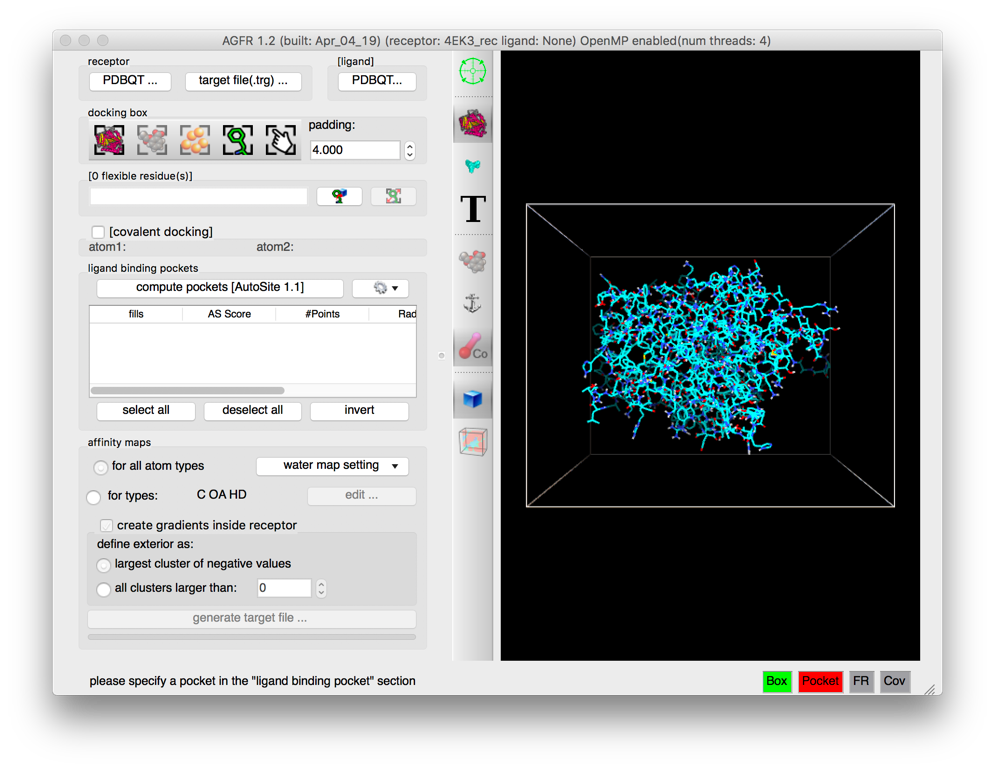
run ADFRsuite-1.0/bin/agfrgui to start the Graphical User interface for these tutorials.
Click  and select 4EK3_rec.pdbqt
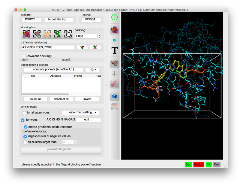
Details: the receptor molecule is loaded and displayed as line representing atomic bonds colored by atom type with carbon atoms shown in cyan. The default docking-box covers the entire receptor with the default padding (4.0 Angstroms) added to each side.
NOTES:
- Amino acids located in the docking box with no flexible side-chains (i.e. glycine, alanine and proline) are displayed with dimmed down lines.
- Several buttons in the control section and the tool-bar are now enabled.
- The status bar indicates that the next step could be to detect pockets.
The 3D scene can be rotated, translated and scaled using the 3 mouse buttons:
| Mouse button | Action |
| Left | Rotate |
| Middle | Translate |
| Right | Scale |
Depth-cueing can be turned on and off by pressing the keyboard key ‘d’ while the mouse pointer is in the 3D view.
Click on the  button to load 1YKR_lig.pdbqt
Details: the ligand molecule appears in the licorice representation with carbon atoms displayed in yellow.

NOTE:
- More buttons are enabled by this operation both in the control panel and in the tool-bar. In particular the button allowing to position and size the box using the ligand
 .
.
Click  to make the docking box cover the ligand, click on
  to focus the 3D scene on the box, and click
 to label residues in the box.
Details: the docking box is now centered on the ligand and scaled to have a 4.0 angstroms padding from the ligand atoms.
The padding can be adjusted using the spin box in the “docking box” section.
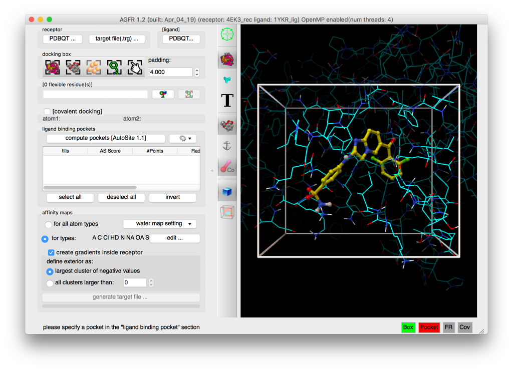
This particular ligand overlaps with side chains of the receptor’s apo conformation. Label the receptor residues in the docking box by clicking in the ![]() button in the tool bar, and zoom in and rotate to observe the overlap of lysine 33 and lysine 89 with the ligand.
button in the tool bar, and zoom in and rotate to observe the overlap of lysine 33 and lysine 89 with the ligand.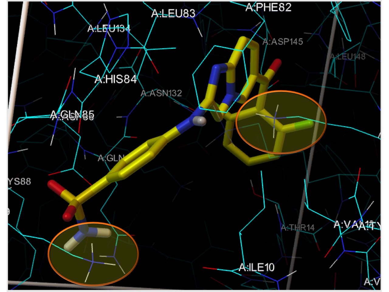
NOTES:
- It is recommended to keep the number of flexible receptor side chains below 15.
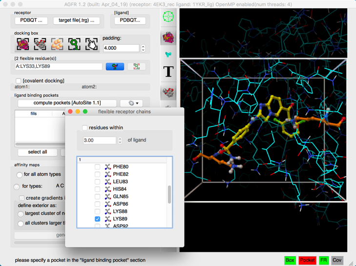
Click on  and select LYS33 and LYS89
Details: a residue selection widget displays all receptor amino acids currently in the docking box and having a side chain that can adopt multiple conformations (i.e. not alanine, glycine or proline). Check the box for a residue select it for having its side chain made flexible during the docking. Side chains selected as flexible for docking are displayed in the 3D view as orange Sticks & Balls and listed in the type in widget.
NOTES:
- If a ligand has been loaded, receptor side chains to be made flexible can also be selected based on their distance from the ligand by checking the “residue within” button. Checking this button will override the current selection with the set of receptor side chains having at least one moving side chain atom within the current distance cutoff (i.e. 3.0 Angstroms in this case) of the ligand. Keep in mind that the more side chains are made flexible the harder the docking problem. While ADFR has no hard limit on how many side-chains can be made flexible we recommend keeping the number below 10 to 15.
- The receptor amino acids selected to have flexible side-chains during the docking calculation are now listed in the type-in widget.
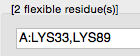 along with the number such residues. Flexible residues can be specified manually by typing directly in this widget. A residue can be specified by its residue number (e.g. “89”), or by its residue type and number (e.g.“LYS89”). Multiple residues must be separated by a comma ‘,’ or space characters, optionally preceded by a chain id (i.e. “A:120,LYS89”). If the chain id is omitted matching residues from all chains are selected. Residues from different chains can be specified by separating the selection string for each chain by a semi colon ‘;’ e.g. “A:10,24,35;B:12,34”
 - Close the interface by destroying the window, using the button in the corner of the window.
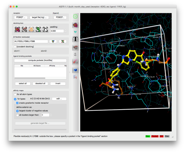
Type “,88” in the type-in widget for flexible residues en press the key
Details:
- one more residue (lysine 88) is selected to be have a flexible side chain during docking.
- the flexible residues and the selection string in expanded.
- the ‘FR’ status light (bottom right of the GUI) turned red (i.e. invalid box)
Click on  to adjust the docking box to cover all flexible receptor atoms
Details:
- the docking box has been extended to fully cover all flexible residues (33, 88 and 89)
- the status light for flexible receptor side chains validity ‘FR’ is now green in the status bar
Click on 
Details: ligand binding pockets are computed using AutoSite by identifying and cluster high affinity points. Each cluster of points is called a “fill” and listed in the table widget. The pocket with the largest AutoSite score is selected by defaults and displayed as a set of green dots. The fill points of all selected fills are displayed in the 3D viewer and will be written into the target files.
NOTES:
- the “Pocket” status light is now green
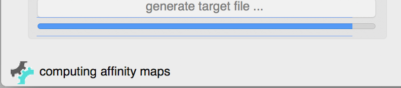
- the “generate target file …” is enabled.
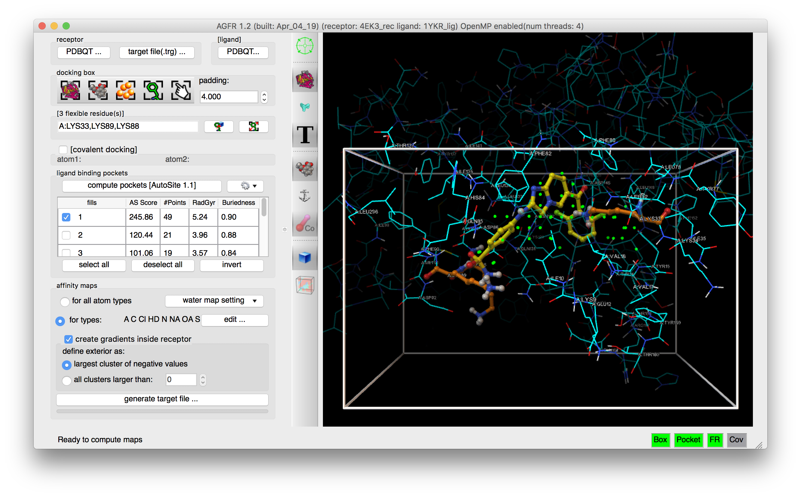
Check the  button
Details: loading the ligand initialized the list of maps to be computed to the list of AutoDock atom types found in the ligand, in this case: “A C Cl HD N NA OA”. Computing maps for all atoms types will use a little more disk space but the resulting target file can be used for any ligand and is recommended.
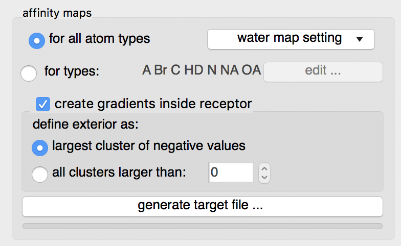
The “edit …” button will display an interface for manually specifying the list of atoms types for which affinity maps are requested.
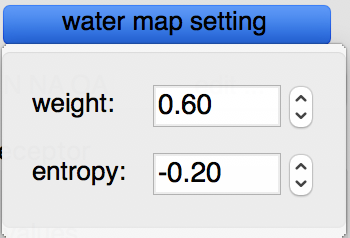
Water maps: water maps are calculated automatically and stored in the target file. These maps allow to perform hydrated docking. the parameter for these maps can be set in the “water map setting” pull down.
Gradients: By default, an affinity gradient will be created for the region of the grid covered by the receptor (except for the electrostatic and desolvation maps). If your CPU has multiple cores and OpenMP is detected, the calculation will execute in parallel and the number of available threads appears in the GUI title bar. Gradients are not required, however, they are recommended as they have been shown to help docking find solutions more efficiently. The addition of gradients requires the definition of the interior and exterior of the receptor. By default, the largest cluster of negative values (favorable affinities) is used to define the exterior of the receptor. In this case, everything else, including receptor cavities large enough to hold solvent but not open to the solvent, will be considered the interior and will be overwritten with the gradient. To prevent the gradient generation on grid points of internal cavities, the user can specify a cluster size above which clusters of points with negative values are considered to be outside the receptor and therefore preserve their original affinity values.
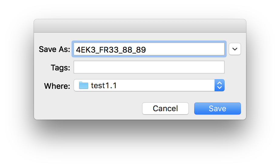
Click on the “generate target file…” button, name the target file as 4EK3_FR33_88_89
Details: the program asks for the name and location for the target file that will be generated. It will then compute the affinity maps and store them in the target file along with meta data.
The generated target file describes the binding pocket targeted for docking on the receptor. It stores the PDBQT file of the receptor used to compute the affinity maps, the grid parameter file used to run AutoGrid, as well as files generated by the AutoGrid run (i.e. affinity maps, AutoGrid log file, etc.). In addition, it stores meta-data about the generation of the target file such as: the time and computer architecture on which the maps were computed, the docking-box parameters, the grid parameter file, the versions of AGFR and AutoSite, the water map parameters, etc.
It is recommended to use names that are descriptive. In this case we use 4EK3_FR33_88_89.
Pressing the “Save” button will start the calculation in a separate thread, leaving the graphical user interface responsive. The progress bar below the button will indicate the level of completion of the calculation.
NOTE: a target file can be inspected from the command line using the about command (AutoDockSuite-1.0/bin/about)